Visualizing Time Series with Gramian Angular Fields (GAF)

Introduction

Time series data is everywhere, from stock prices and sensor readings to ECG signals. While traditional models like ARIMA and LSTMs are powerful, what if we could leverage the incredible success of Convolutional Neural Networks (CNNs), which excel at image recognition, for time series analysis?

This is where Gramian Angular Fields (GAF) come in. GAF is a novel technique that encodes a one-dimensional time series into a two-dimensional image. This transformation allows us to apply powerful deep learning models like CNNs to time series classification and regression tasks.

There are two main types of GAFs:

Gramian Angular Summation Field (GASF)
Gramian Angular Difference Field (GADF)

In this post, we’ll dive into the mechanics of how GAFs work and show you how to implement them in Python.

How Do Gramian Angular Fields Work?

The process of converting a time series into a GAF image involves a few clever steps. Let’s break it down.

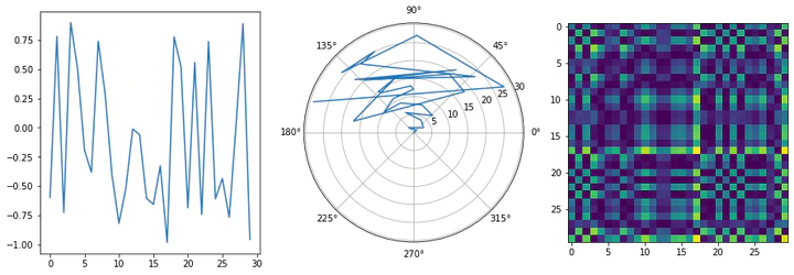
Step 1: Rescale the Time Series

First, we need to rescale the time series values to a uniform range. This is typically done to fit the values within the domain of trigonometric functions, for example, scaling to [-1, 1] or [0, 1].

Step 2: Convert to Polar Coordinates

Next, the rescaled time series is represented in a polar coordinate system. Each rescaled value x̃ᵢ is converted into an angle φᵢ by taking its arccosine (φ = arccos(x̃ᵢ)). The timestamp tᵢ serves as the radius.

This step is the core of the technique, as it encodes the temporal information (the timestamp) and the value into a polar representation.

Step 3: Calculate the Gramian Matrix

The final step is to compute the Gramian matrix from these polar coordinates. This is done by considering the trigonometric sum or difference of the angles.

For the Gramian Angular Summation Field (GASF), the matrix is computed as: GASF = [cos(φᵢ + φⱼ)] The GASF matrix identifies the temporal correlation by leveraging the cosine sum.
For the Gramian Angular Difference Field (GADF), the matrix is computed as: GADF = [sin(φᵢ - φⱼ)] The GADF matrix is useful for preserving temporal dependencies through the sine difference.

The resulting matrix is a GAF image, where each pixel (i, j) represents the relationship between the time points i and j.

Implementation in Python

You don’t have to implement this from scratch. The pyts library in Python provides an easy-to-use implementation of GAF.

First, you’ll need to install pyts:

pip install pyts

Here’s a simple code snippet to generate GASF and GADF images from a sample time series:

import numpy as np
import matplotlib.pyplot as plt
from pyts.image import GramianAngularField

# 1. Create a sample time series
time_series = np.array([0.1, 0.5, -0.2, -0.8, 0.4, 0.9, 0.2, -0.5])

# 2. Reshape for pyts
X = time_series.reshape(1, -1)

# 3. Create GASF and GADF images
# Method can be 'summation' or 'difference'
gasf = GramianAngularField(image_size=8, method='summation')
X_gasf = gasf.fit_transform(X)

gadf = GramianAngularField(image_size=8, method='difference')
X_gadf = gadf.fit_transform(X)

# 4. Plot the results
fig, axes = plt.subplots(1, 2, figsize=(10, 5))
axes[0].imshow(X_gasf[0], cmap='rainbow', origin='lower')
axes[0].set_title('GASF')
axes[1].imshow(X_gadf[0], cmap='rainbow', origin='lower')
axes[1].set_title('GADF')
plt.show()

This code will produce two 8x8 images representing the GASF and GADF of the input time series.

Applications and Advanced Usage

GAFs have been successfully applied in various domains, including:

Finance: Predicting stock market movements by converting price charts into images.
Healthcare: Classifying ECG or EEG signals for medical diagnosis.
Industrial IoT: Detecting anomalies in sensor data from machinery.

Leveraging CNNs with GAF

The primary advantage of transforming time series into GAF images is to harness the power of Convolutional Neural Networks (CNNs). CNNs are exceptionally good at learning spatial hierarchies of features from images. When applied to GAF images, CNNs can automatically extract complex patterns and relationships within the time series that might be difficult to discern using traditional time series analysis methods. This makes them particularly effective for tasks like:

Classification: Identifying different states or events within a time series (e.g., classifying types of heartbeats from ECG data).
Anomaly Detection: Pinpointing unusual patterns that deviate from normal behavior.

Beyond using GAF images alone, this technique can be integrated into multi-modal learning approaches. In scenarios where you have multiple types of data (e.g., sensor readings, video, audio), GAF can convert time-series components into an image format. These GAF images can then be combined with other data modalities (e.g., raw sensor data, features extracted from other modalities) and fed into a multi-modal deep learning model. This allows the model to learn from the rich, complementary information provided by different data representations.

For instance, in a project like FogSense (a hypothetical example for context), which might involve monitoring environmental conditions using various sensors, GAF could be used to convert individual sensor time series into images. These GAF images, along with other environmental data (e.g., humidity, temperature, air quality), could then be fed into a multi-modal model to predict fog formation or other atmospheric events. This approach allows for a more comprehensive understanding of complex phenomena by integrating diverse data sources.

Conclusion

Gramian Angular Fields provide a powerful and intuitive bridge between the worlds of time series analysis and computer vision. By transforming temporal patterns into images, GAFs unlock the potential to use state-of-the-art CNN architectures for tasks that were traditionally handled by other models. Furthermore, their compatibility with multi-modal learning paradigms significantly expands their applicability, allowing for richer insights from diverse datasets. This technique is a valuable addition to any data scientist’s toolkit for tackling complex time series problems.